Assalamu’alaikum & Howdy Folks!
In this entry I would like to illustrate certain forms of data exploration. Normally, one of the first steps that you need to perform would be EDA or Exploratory Data Analysis. You have these vast amounts of data but you do not yet have a problem statement nor do you have an idea what story are all those data trying to tell you.
Due to the sheer enormity of the data, I had divided them into several (still very huge) chunks. Each about a thousand records out of over 49,000 rows or records or observations.
I exported the data into csv format (I tried json but in this particular case csv works much better). If I had used the json format, there’s an additional step to convert the data into useful data frames, at least one extra step. With csv, the data will be nicely imported into R in the form of data frames which I had wanted.
Tools we need: RStudio (we’ll be using R exclusively)
Some of the Techniques used:
Topic Modeling (https://en.wikipedia.org/wiki/Topic_Model)
Latent Dirichlet Allocation (https://en.wikipedia.org/wiki/Latent_Dirichlet_Allocation)
Part-of-Speech Tagging (POS Tagging)
Ngrams(mostly Bigrams)
Word Clouds
Pointwise Mutual Information ( https://en.wikipedia.org/wiki/Pointwise_mutual_information)
Rapid Automatic Keyword Extraction (https://hackstage.haskell.org/package/rake).
You can request for the data set by emailing us 
We have been aggregating these data for the past several years and now is the time to dig some of the stories for your reading pleasure.
What better way to speculate what content than inspecting the title itself.
My method eliminates the need for several text pre-processing and text processing thus, again, I had minimised the process which derived a more desirable format of data.
	for(a in 1:nrow(news))
{
  page <- as.character(news$html[a])
  htmlpage <- read_html(page)
  headlines <- html_text(html_nodes(htmlpage, "title"))
  news$headlines[a] <- headlines
}
The approach I used was to make use of un-scraped data which still is in html format. As the code above depicts, I had used the html title tag to extract the titles of each of the articles. You may have noticed that this is one easy way to actually mine the actual topics without having to use proper topic modelling methods.
	for(i in 1:nrow(news))
{
  page <- as.character(news$html[i])
  htmlpage <- read_html(page)
  para <- html_text(html_nodes(htmlpage, "p"))
  news$para[i] <- para
}
It turns out that some of the articles on Johor does not have the “Johor” keyword in the title itself. Thus, there are more data which we can work with. On that note, we will include those data as well.
Thus, I had also extracted data from the p tags which forms the bulk of the content. This way I didn’t have to perform text pre-processing, removing punctuations, special characters, JavaScript codes, stopwords and so on and so forth. Everything was achieved by pretty much a single step. See the code snippet above.
There are many ways to filter the data and I had used more than three different types. Anyway, I hope this particular method will be easy to understand.
	Library(sqldf)
johordata <- sqldf("select * from news where text like '%ohor%'")
I intentionally used “ohor” instead of “Johor” or “johor” since that way the code will be inclusive. Of course, you can convert everything to lowercase and filter for “johor”.
Now that we have a list of the titles, let’s filter them so that we only see ones which refers to Johor.
I had filtered the data set chunks to only obtain news articles that contain the keyword “Johor”. Subsequently, I had merged them into one huge data set. Thus, I have thousands of news articles that mentions “Johor”
Now that we have a filtered list, let’s get acquainted with a technique called Topic Modelling.
One common method is to use TF-IDF (Term Frequency-Inverse Document Frequency) method to extract the latent news topics but I would not cover that method within this post.
Another (more common) method is to use Latent Dirichlet Allocation or LDA in short. The acronym LDA also is used to refer to another method called Linear Discriminant Analysis which we won’t address this time around.
R has a specific package for topic modelling called topicmodels.
Next, we convert the data into a corpus to be used with the package.
		library(tm)
docs <- Corpus(VectorSource(johordata))

docs <- tm_map(docs, removeWords, stopwords("english"))
docs <- tm_map(docs, tolower)
docs <- tm_map(docs, removeWords, stopwords("english"))
docs <- tm_map(docs, removeWords, "the")
docs <- tm_map(docs, removeWords, c("today", "abdul", "malaysiakini",
                                    "said","yang","year","says"))
docs <- tm_map(docs, removeWords, c("lagi", "nan", "kini",
                                    "kinilens","may","will","kiniguide"))

docs <- tm_map(docs, tolower)

dtm <- DocumentTermMatrix(docs)
freq <- colSums(as.matrix(dtm))
length(freq)
ord <- order(freq,decreasing = T)
freq[ord]
Consequently, let’s mine for the topics and create the visualisation to have an idea of what the topics were.
	library(topicmodels)

johordata_lda <- LDA(dtm, k=5,control = list(seed=1234))

library(tidytext)

johordata_topics <- tidy(johordata_lda,matrix="beta")

library(ggplot2)

johordata_top_terms <- johordata_topics %>%
  group_by(topic) %>%
  top_n(10,beta) %>%
  ungroup() %>%
  arrange(topic, -beta)

johordata_top_terms %>%
  mutate(term=reorder(term,beta)) %>%
  ggplot(aes(term,beta,fill =factor(topic))) +
  geom_col(show.legend = F) +
  facet_wrap(~ topic, scales="free") +
  coord_flip()
In the code snippet above, I had specified 5 topics to be extracted:
johordata_lda <- LDA(dtm, k=5,control = list(seed=1234))
You can specify the number of topics by specifying an integer value to k.
Subsequently we will use Latent Dirichlet Allocation (LDA) to perform topic modelling.
johordata_top_terms
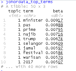
This has turned the model into a single topic per row per term format. In each combination, the model computes the probability of that term being generated from that topic. For instance, the term “warisan” has a 0.00570 probability of being generated from topic 1. We know that the term actually refers to the political party. Later we will use Parts of Speech (POS) tagging methods to inspect the grammatical classifications of the words for more meaningful analysis. This method will also extract named entities such as individuals, political parties or other organisations.
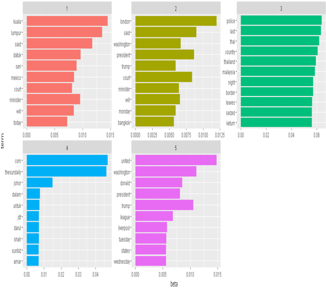
From the visualisations above, we can derive that the of the news on Johor is related to a multitude of areas. In other words, the latent topics the news articles harbour. The first topic may refer to political or diplomatic issues with Mexico, the second topic covers an international news item probably involving President Trump’s visit to Thailand, the third topic is very clear in which it’s about the smuggling of ketum to Thailand, the fourth may refer to sports and finally the fifth may refer to President Trump’s interest in Soccer or soccer clubs. Only the fourth news is probably really related to Johor in this case. However, to obtain more latent information, you can increase the value of k in your LDA code.
Let’s take a look at the top ten most frequent words:
Issue this command
| malaysia | malaysia | 303 |
| police | police | 260 |
| last | last | 258 |
| country | country | 256 |
| thai | thai | 252 |
| thailand | thailand | 251 |
| night | night | 232 |
| border | border | 232 |
| leaves | leaves | 229 |
| ketum | ketum | 228 |
Looks like ketum may be a notable issue to be reckoned with.
After performing a Parts of Speech Tagging (POS Tagging), we found out that proper nouns are most frequent, followed by general nouns.
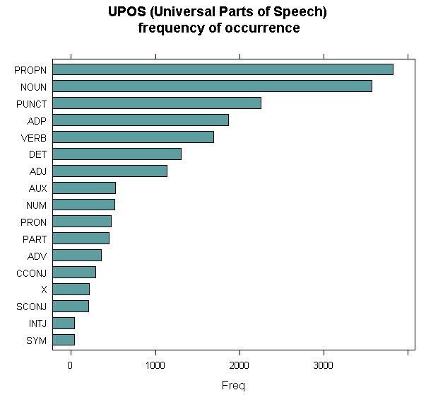
A proper noun is a name used for an individual person, place, or organization, spelled with an initial capital letter, e.g. Jane, London, and Telekom Malaysia.
Nouns are the second most frequent words present in those articles. We will investigate what those nouns are later.
First, let’s take a look at 20 of the most frequently occurring proper nouns.
	library(lattice)
stats <- txt_freq(y$upos)
stats$key <- factor(stats$key, levels = rev(stats$key))
barchart(key ~ freq, data = stats, col = "cadetblue",
         main = "UPOS (Universal Parts of Speech)\n frequency of occurrence",
         xlab = "Freq")

stats <- subset(y, upos %in% c("PROPN"))
stats <- txt_freq(stats$token)
stats$key <- factor(stats$key, levels = rev(stats$key))
barchart(key ~ freq, data = head(stats, 20), col = "cadetblue",
main = "Most frequent prepositions", xlab = "Freq")
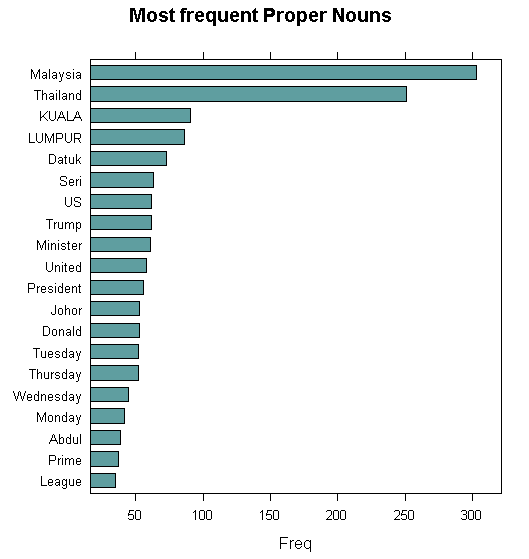
A lot of these proper nouns are political in nature; thus, we can conclude that one of the latent commonly covered news is political.
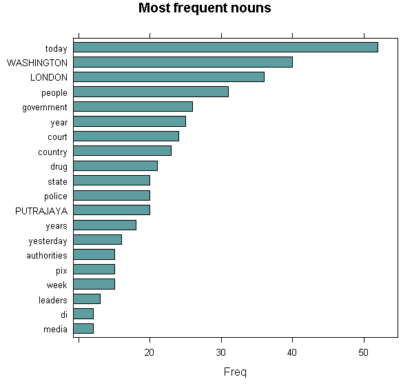
The most frequent nouns however, seems to refer to criminal and enforcement activities.
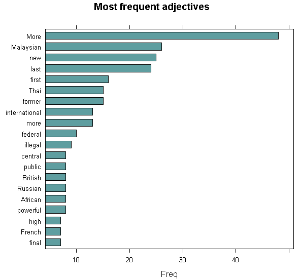
Adjectives explains or modify nouns. They give a more meaningful understanding of nouns. From the figure above, it looks as though the criminal activities and enforcements were mostly international. Since Thai is rather frequent, they probably refer to the ketum smuggling to that country. Still, not much relevant to Johor unless probably Johoreans were involved in either enforcement or illegal activities.
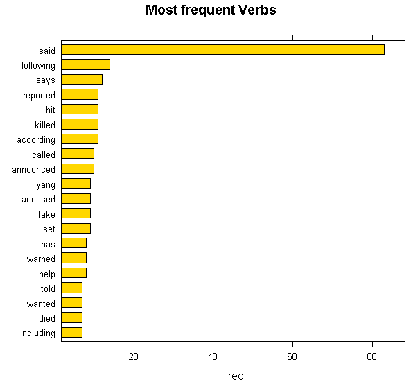
Here’s a code to visualize the usage of verbs.
	stats <- subset(y, upos %in% c("VERB"))
stats <- txt_freq(stats$token)
stats$key <- factor(stats$key, levels = rev(stats$key))
barchart(key ~ freq, data = head(stats, 20), col = "gold",
         main = "Most frequent Verbs", xlab = "Freq")
Verbs usage tells a story. Most popular verbs here points to criminal activity.

The word cloud shows that the news is overwhelmingly about the ketum problem in terms of coverage.
In order to inject a little bit of fun, I had used wordcloud2 package which has more features than word cloud in which I can use the Johor map as a backdrop and the word cloud will take the shape of the Johor map. Previously that package worked fine but recently there’s a bug the package developer has not fixed (https://github.com/Lchiffon/wordcloud2/issues/12).
It would be nicer if the bug I mentioned were fixed.
Next, let’s perform a Parts of Speech Tagging on the content of the news articles. We will use a package called udpipe. Another useful package for text mining (apart from tm) is quanteda. Definitely there are several other NLP packages you can use but I’m not going to cover them in this post.
	library(udpipe)
#model <- udpipe_download_model(language = "english")
udmodel_english <- udpipe_load_model(file = 'english-ud-2.0-170801.udpipe')
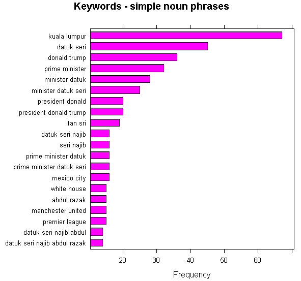
A simple noun phrases analysis will show you that most articles were political and diplomatic and received more coverage that say, sports. But being in the top 20 the EPL and Manchester United seems to also garner so much attention that warrants them to be frequently covered.
Let’s try to use PMI using this code:
	## Using Pointwise Mutual Information Collocations
y$word <- tolower(y$token)
stats <- keywords_collocation(x = y, term = "word", group = "doc_id")
stats$key <- factor(stats$keyword, levels = rev(stats$keyword))
barchart(key ~ pmi, data = head(subset(stats, freq > 3), 20), col = "cadetblue",
         main = "Keywords identified by PMI Collocation",
         xlab = "PMI (Pointwise Mutual Information)")
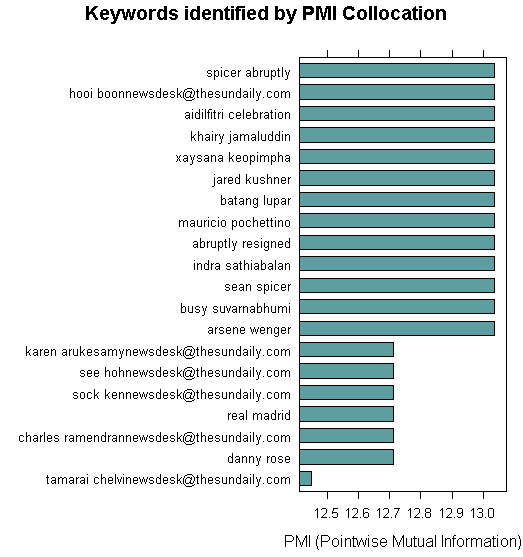
Apparently not much can be told from the PMI. It mostly shows who are the most prolific reporters with some reference to politicians and political events.
Now we will examine the relationship between nouns and verbs, basically who is doing what.
	#Visualizing Cooccurrence of Nouns & Adjectives within sentences
library(igraph)
library(ggraph)
library(ggplot2)
wordnetwork <- head(cooc, 30)
wordnetwork <- graph_from_data_frame(wordnetwork)
ggraph(wordnetwork, layout = "fr") +
  geom_edge_link(aes(width = cooc, edge_alpha = cooc), edge_colour = "pink") +
  geom_node_text(aes(label = name), col = "darkgreen", size = 4) +
  theme_graph(base_family = "Arial Narrow") +
  theme(legend.position = "none") +
  labs(title = "Cooccurrences within sentence", subtitle = "Nouns & Adjective")
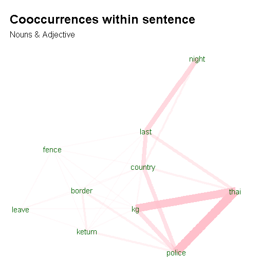
We can see that there are relationships between police and thai and kg (short for kampung) – indicative of PDRM’s actions against the smuggling of ketum leaves to Thailand via rural village routes?
Next, we analyse verbs and nouns that follow each other.
	#nouns / adjectives which follow one another
cooc <- cooccurrence(x$lemma, relevant = x$upos %in% c("NOUN", "ADJ"), skipgram = 1)
head(cooc)
library(igraph)
library(ggraph)
library(ggplot2)
wordnetwork <- head(cooc, 15)
wordnetwork <- graph_from_data_frame(wordnetwork)
ggraph(wordnetwork, layout = "fr") +
  geom_edge_link(aes(width = cooc, edge_alpha = cooc)) +
  geom_node_text(aes(label = name), col = "darkgreen", size = 4) +
  theme_graph(base_family = "Arial Narrow") +
  labs(title = "Words following one another", subtitle = "Nouns & Adjective")
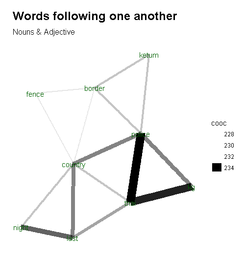
By analysing nouns and adjectives that follows one another (remember, adjectives and attributive nouns explains or modify nouns) we derive a very similar visualization which points to illegal ketum trade activities cross different countries. It involves smuggling over border fences dividing Malaysia and Thailand and happens mostly (if not exclusively) at night time.
Next, I had created a bigrams frequency data frame.
	library(ngramrr)
newsbigrams <-ngramrr(news$para,char=F,ngmin=2,ngmax=2,rmEOL=T)
stats <- txt_freq(newsbigrams)
stats <- select(stats,keyword,freq)
statssorted <- stats[order(-stats$freq),]
barchart(keyword ~ freq, data = head(stats,17), col = "red",
         main = "Bigrams frequency", xlab = "Frequency")
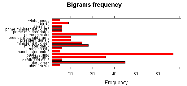
	From the bigrams, we could see that the Prime Minister was frequently, so was Manchester United.

Finally, I had calculated how many times the keyword “Johor” had occurred in each of the articles. Assuming the ones with the most number of (Johor) keywords are the most relevant to Johor.

[1]   Political animals gnaw at apostasy issue | Free Malaysia Today
[2]   Johor Bahru | Free Malaysia Today
[3] Perlawanan akhir Piala Malaysia 2014 | Foto | Astro Awani
[4]   Here’s why Dr Mahathir is taking on the Sultan of Johor | Free Malaysia Today
[5]   ‘Taiko’ DAP punca perbalahan pembangkang | Free Malaysia Today
[6]   Four questions for the Johor Govt about the VEP | Free Malaysia Today
Again, the bulk of the news were political followed by sports, showing Malaysians interest in both, in that order. As explained earlier, the articles explicitly mentions Johor in their content, as can also be seen in the articles that frequently mentions Johor by name.
Coming Up Next Week!
Is Kit Siang more popular than Tun Dr Mahathir?
Are Johoreans involved in Ketum trade and smuggling?