I am not particularly an avid soccer fan but recent developments in our country’s soccer, seemingly spearheaded by JDTFC and the TMJ has raised my interest in performing certain analysis in regards to JDTFC or more fondly known as simply, JDT (henceforth, will be referred to as such).
The recent ascent of JDT in world rankings may probably have somewhat chagrined certain quarters, especially fans of competing clubs, as a result of jealousy (tounge-in-cheek).
AFC Club Ranking
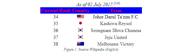
As of July, 2017, JDT’s Asian ranking have even surpassed that of Japanese and Korean as well as New Zealand’s clubs.
Thus our problem statement is concerned about what do Johoreans really feel about JDTFC simplified to “Johoreans do not like JDTFC that much” just to stoke your interest.
In order to validate whether or not JDT have that many fans, or anti-fans, or people who simply dislike JDT, we have put together a series of data visualizations as a result of our analysis and we conclude that, well, let’s go through with them first.
First order of business would be determining where to obtain enough data for our analysis.
In view of the constraints of circumstance, we had decided to crawl and mine twitter data available concerning our lovely soccer landscape. In order to perform many types of analysis and to process the data through analytics and various established algorithms, it has to be in English. Malay language NLPs (Natural Language Processing) for instance, is practically non-existent, yet. Take for example, a procedure for performing sentiment analysis, it would require a comparison of words against dictionaries which had already assigned sentimental values to them. This is not yet sufficiently available in Malay.
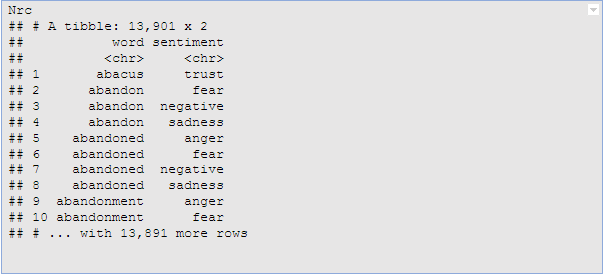
For example, consider the NRC Word-Emotion Association lexicon, available from the tidytext package, which associates words with 10 sentiments: positive, negative, anger, anticipation, disgust, fear, joy, sadness, surprise, and trust.
Hence, more work is still needed to be able to comfortably perform sentiment analysis for Malay language text. We employed various dictionaries including syuzhet, Harvard IV, bing, afinn, nrc and several others, all of which caters only for English.
We are not only talking about sentiment analysis but NLP (Natural Language Processing) as a whole. NLP in IT terminology is a subset of AI (Artificial Intelligence) of which programs and computers were built to be able to “understand” human languages as humans do. These kinds of capabilities are very much new and scarce as far as the Malay language is concerned.
Subsequently, the Malaysian twitter community is steadily growing and projected to continue to grow.
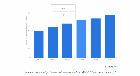
As of 2017, there are about 2.1 million ACTIVE Malaysian twitter users and the figures are steadily increasing.
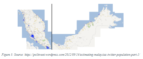
In terms of population distribution, most Malaysian twitters are located in Kuala Lumpur as well as Johor Bahru.
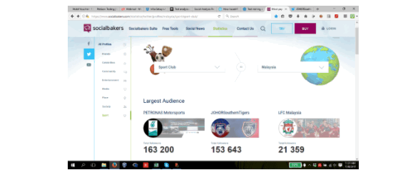
According to socialbakers.com, the most popular twitter channel for Malaysian soccer is officialjohor, leaving Liverpool Malaysian fans channel FAR behind at leaps and bounds to number two.
https://www.socialbakers.com/statistics/twitter/profiles/malaysia/sport/sport-club/
Subsequently, we crawled the latest data in 2017 and saved in in CSV format for easier wrangling.
You can also obtain the data from our website:
http://ilokensystem.net/files/JDTFC_Dataset.csv
Once the data has been loaded up, we perform a number of analysis, with the help from our trusty, popular and free analytics tool, R.
We then proceed to perform a sentiment analysis based on the tweets.
The dataset
First we’ll retrieve the content of officialjhor’s timeline using twitter crawler written in Python below;
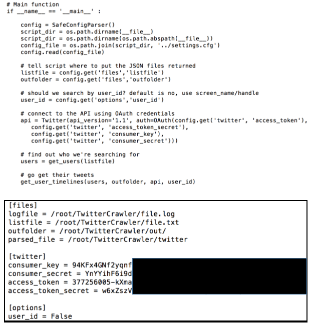
Click this link https://github.com/shaiful-hisham/JDTTwitterCrawler to get the source code like above
All the secret keys will be written in the configuration file. For example, I have created a setting.cfg file and put all files path and twitter secret keys in it.
Referring to the above code, in order to create the token keys, you will need a working twitter id which has also been linked to your mobile number.
Browse to https://apps.twitter.com/ and create an application from there.
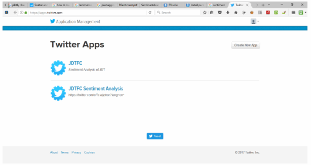
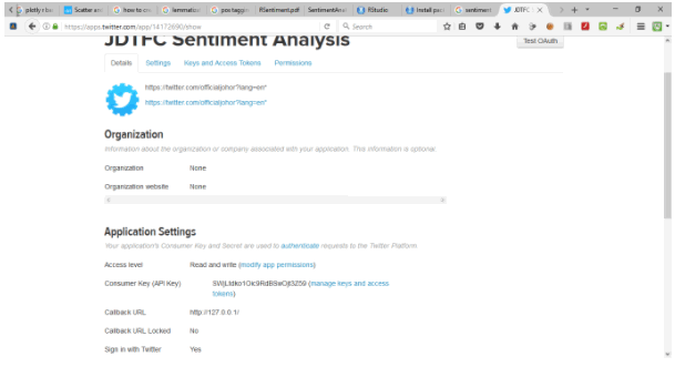
The figures above are just examples. The keys that needs to be supplied to the R code will be created from that site. There are various step-by-step guides available and we will be concocting our own guide later and will be sharing it with the rest of the world through our website.
Once we have obtained the data, let’s perform a simple, quick sentiment analysis on the data. We can achieve this using many ways, different algorithms and many different R functions and libraries. But for our case, we will just try one of the simplest ways to do just that. But before we proceed, let’s investigate a tiny bit into the philosophy and approach in performing this sentiment analysis.
Our field of interest will be the actual tweet text which was aptly named well, tweet_text! Our approach will be by analysing the rows, or record entries, we look for certain key words that carries positive, negative or neutral connotations. Tweets that contain words or text like “congratulations” and “GOAL” will be given a score of 1, denoting a positive and words like “misses” will have a negative reflection. You get the idea. The approach will be by assigning a -1, 0 or 1 for each of the rows respectively reflecting whether they are negative, neutral or positive comments or tweets. Alternatively, we can use the script below to perform the analysis of which numeric values will be assigned to each cell. Consequently, by applying certain commands, those values can be converted to “positive”, “negative” and “neutral”.
The script to do this is shown below:
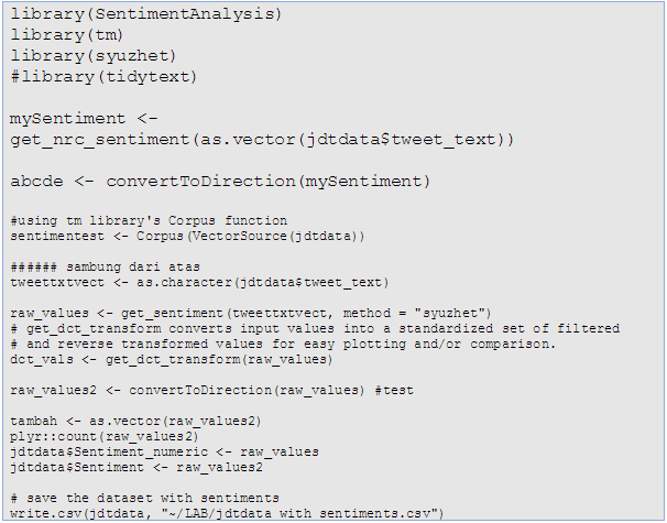
Now that we have the sentiments assigned, we will add it to the records in an additional column we call Sentiment.
Now let’s take a look at how many tweets has been posted separated by likes and dislikes.
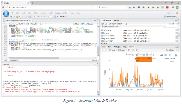
Let’s zoom it up a bit:
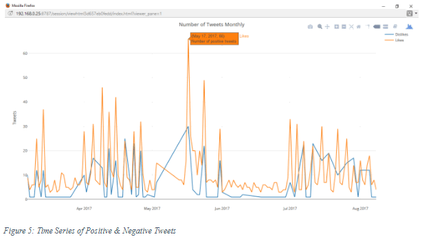
The orange line indicates how many positive tweets over the course of several months up until August 2017. The blue line indicates negative comments. The peaks on both lines corresponded very well with dates when matches took place, an indication that most likely a match involving JDT will trigger a heightened interest to tweet. You may argue that the number of tweets may be contributed by followers who actually do not like JDT. Our argument is that if they don’t like JDT why then, would they follow the channel. The negative feedbacks was due to sentiments such as missed opportunities, disagreeing with the referee and so forth. You can hover your mouse to each of the peaks to see the exact date they represent.
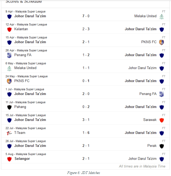
Here’s a list of matches involving JDT for your reference:

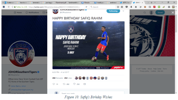
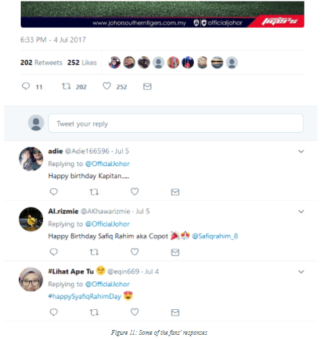
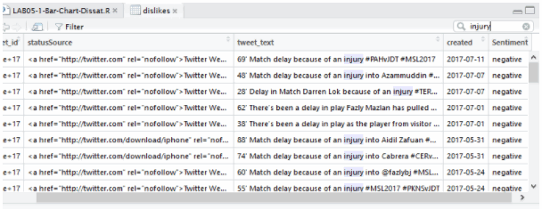
Let’s take a look at some of the positive comments:
From RStudio, search for birth as the keyword to find tweets about birthday wishes and announcements:
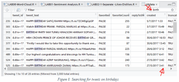
Scroll to the right to see the Sentiment:
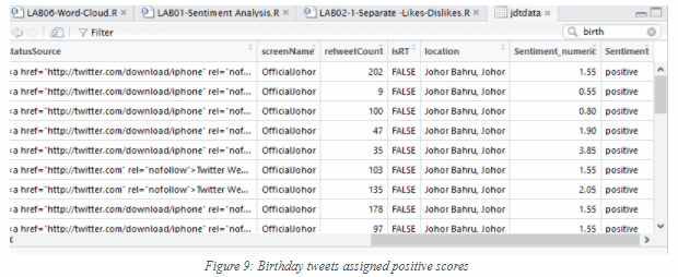
Would you greet the persons you hate with a birthday wish, even more so in public?!
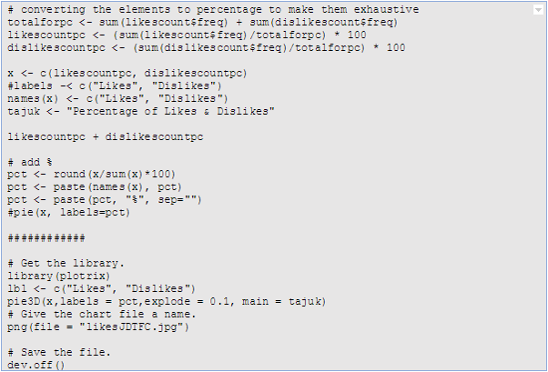
Now let’s take a peek at a pretty generic display of likes and dislikes – pie chart. In order to achieve this, we concocted this R script which we share in the box below:
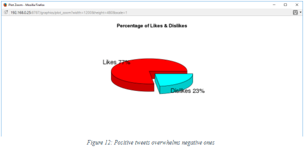
The “likes” are overwhelmingly larger than the dislikes, indicating a possible greater number of fans than anti-fans.
Would you like to know who’s the most talked about player? Let’s create a word cloud for us to find that out. But prior to that, do understand that tweet text also contains words that we do not want to count such as stop words, URLs and junks.
We need to clean up the text a bit.
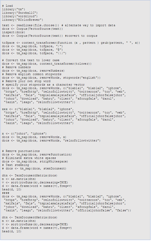
Let’s go about clearing the stop words first. Oh! What are stop words? They are common words like “to”, “from” “with”, well, the list goes on. We’ll show you the command if you would like to see the list of standard English stop words in a fair bit.
We will need to clean the texts from stop words, extra spaces, punctuations, garbage and so forth. Here’s the script to do just that:
Let’s move on to investigate further on the negative posts. We now extract ONLY the negative tweets of about 23% of the whole posts. We further classify them based on Naïve Bayes classifier to three distinct posts namely, management, facilities and the game itself. We group them further together into the three entities we mentioned. This is called agglomerative clustering where it involves clustering of an existing cluster. Agglomerative clustering also involves a structure or hierarchy, in this case, sentiment, then the three entities. Games would most usually mention players who are also entities but we group them together with game for our analysis.
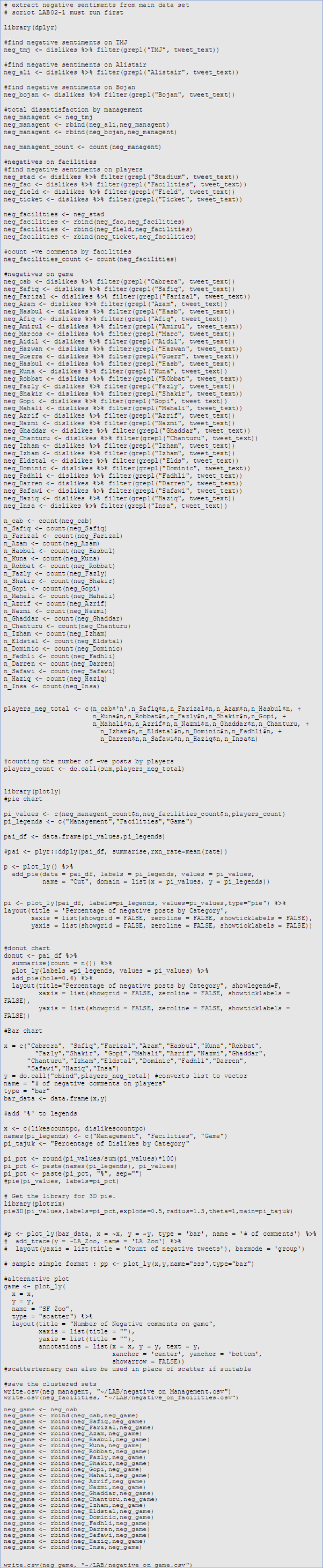
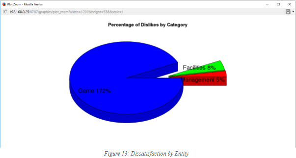
The negative posts are mostly on the game itself such as missed opportunities, yellow cards and so forth.
Finally, we save the best for last. Let’s find out who is the most talked about player a.k.a the most popular.
The code to produce a word cloud is shown below:
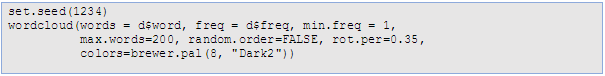
You can reuse these codes if you like, with different datasets.
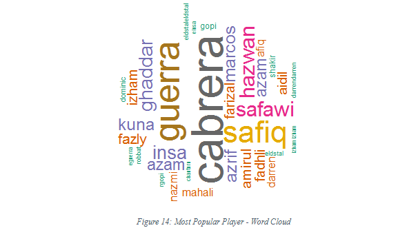
Now that we’ve seen the word cloud, we’ll be able to see the most frequently mentioned player in the tweets. Cabrera obviously is the most popular word and the most talked about thus, we can conclude that Cabrera is the key word that garners the most interest.
Thus we conclude that Johoreans really do love JDT, MUCH more so than any other soccer fans in Malaysia.